Category:Dynamical systems
Przejdź do nawigacji
Przejdź do wyszukiwania
English: Dynamical systems deals with the study of the solutions to the equations of motion of systems that are primarily mechanical in nature; although this includes both planetary orbits as well as the behaviour of electronic circuits and the solutions to partial differential equations that arise in biology. Much of modern research is focused on the study of chaotic systems.
mathematical model which describes the time dependence of a point in a geometrical space  | |||||
| Prześlij plik multimedialny | |||||
| Jest to |
| ||||
|---|---|---|---|---|---|
| Podklasa dla | |||||
| Składa się z | |||||
| |||||
Podkategorie
Poniżej wyświetlono 27 spośród wszystkich 27 podkategorii tej kategorii.
*
A
B
- Brusselator (9 plików)
- Bunimovich stadiums (4 pliki)
C
D
H
I
L
O
P
- Pentagram maps (18 plików)
- Poincare map (11 plików)
S
- Simple harmonic motion (35 plików)
T
Pliki w kategorii „Dynamical systems”
Poniżej wyświetlono 186 spośród wszystkich 186 plików w tej kategorii.
-
 080205 Brusselator picture.jpg 629 × 380; 25 KB
-
 2397.png 1386 × 1000; 38 KB
-
 3000.png 1386 × 1000; 73 KB
-
 3869.png 1386 × 1000; 39 KB
-

-
 Adaptive-cycle.png 1620 × 1095; 312 KB
-

-
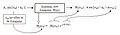
 Analyse grenzschwingungen im zweiortskurvenverfahren.png 867 × 443; 32 KB
-
 Arnold tongues.png 1500 × 378; 21 KB
-
 AsymptoticStabilityImpulseScilab.png 530 × 270; 4 KB
-
 B&S-1-tipped.jpg 789 × 731; 34 KB
-
 Ba model 1000nodes.png 871 × 850; 650 KB
-
 BasicLMIregions.pdf 1041 × 610; 32 KB
-
 Before after dynamical systems definition.jpg 601 × 527; 86 KB
-
 Belousov-Zhabotinsky Reaction Simulation Snapshot.jpg 300 × 300; 35 KB
-
 Bernoulli-shift.svg 485 × 245; 98 KB
-
 Bifurcation diagram of saddle node bifurcation.png 1625 × 605; 59 KB
-
 Bode amplitude.jpg 492 × 243; 24 KB
-
 Bode fase.jpg 498 × 214; 27 KB
-
 Bowen example (heteroclinic attractor).png 599 × 335; 28 KB
-
 Bowen example (heteroclinic attractor).svg 151 × 84; 7 KB
-
 Canard cycles on the two-torus (slides, I. Schurov).pdf 754 × 566, 38 stron; 659 KB
-
 Cauliflower.png 640 × 640; 5 KB
-
 Chaotic regime.png 432 × 288; 40 KB
-
 Coexisting Attractors.png 3000 × 1600; 957 KB
-
 Compensazione.png 772 × 543; 13 KB
-
 Consumer Resource Models Resource Dynamics Schematics.png 1736 × 1372; 424 KB
-
 Contours in the vector field f(z) = -Cos(z).jpg 500 × 231; 173 KB
-
 Counterexamplestability2.svg 356 × 348; 4 KB
-
 CriticalHyperplane.png 445 × 282; 3 KB
-
 Denjoy-example.svg 482 × 473; 91 KB
-
 Diagram of SIR epidemic model states and transition rates.svg 533 × 55; 19 KB
-
 Different attractors in same system.png 800 × 565; 25 KB
-
 Distance between repetitive squaring of point smaller then one.svg 1000 × 1000; 14 KB
-
 DistanceToFixed.png 1000 × 500; 21 KB
-
 DistanceToFixed.svg 1000 × 500; 202 KB
-
 Double well langevin.pdf 1200 × 900; 6 KB
-
 Double-pendulum.png 480 × 547; 47 KB
-
 Douday rabbit rough dynamics.png 800 × 600; 14 KB
-
 Dynamic system.png 248 × 116; 748 bajtów
-
 Envelope astroid.svg 600 × 480; 264 KB
-
 Envelope cast.svg 600 × 480; 117 KB
-
 Envelope string art.svg 600 × 480; 88 KB
-
 Es6p3.png 296 × 385; 5 KB
-
 Example of application of Poincaré–Bendixson theorem.png 415 × 580; 64 KB
-
 Explanation-of-the-nature.png 427 × 563; 22 KB
-
 Explanatory diagram of periodic point.svg 524 × 372; 35 KB
-
 Exponential Stability Estimate of Symplectic Integrators for Integrable Hamiltonian Systems.pdf 1239 × 1754, 32 strony; 263 KB
-
 Figura-4.png 2000 × 2026; 332 KB
-

-
 Fitzhugh-nagumo b = 2.0, separatrix.png 1260 × 1297; 958 KB
-
 Fitzhugh-nagumo b = 2.0, with stable and unstable manifolds marked.png 1314 × 1321; 505 KB
-
 Flow and orbit of vector field (dynamical system).png 590 × 276; 32 KB
-
 Folded-towel map attractor.png 2345 × 2330; 3,42 MB
-
 Four Limit Cycles in Two-Dimensional Polynomial Quadratic System.gif 800 × 564; 151 KB
-
 Fubini Nightmare foliation Katok example.svg 720 × 720; 1,62 MB
-
 Function-block-harmonic-balance.png 1242 × 300; 7 KB
-
 Funções de fase.png 317 × 208; 5 KB
-
 GR inv set iter.png 600 × 600; 9 KB
-
 Grafico exemplo linear.png 548 × 188; 4 KB
-
 Hands HKB in phase fingers.png 646 × 780; 1,25 MB
-
 Hartman-grobman fig1.PNG 506 × 422; 9 KB
-
 Hartman-grobman fig2.PNG 506 × 414; 7 KB
-
 Henon3D.pdf 1104 × 860; 2,23 MB
-
 Henonatrat-eps-converted-to.pdf 1045 × 456; 469 KB
-
 HenonMap.svg 720 × 540; 9,09 MB
-
 Homoclinic and Heteroclinic Connections updated 2020-01-29.svg 741 × 551; 40 KB
-
 Human interactome.jpg 600 × 481; 95 KB
-
 Hyperbolic flow example, illustrating stable and unstable manifolds.png 692 × 665; 309 KB
-
 Illustration of the Propagation of an Ensemble by a Flow.png 1885 × 1079; 152 KB
-
 Intermittency in logistic map, cobweb diagram.png 567 × 455; 42 KB
-
 Intermittency in logistic map.png 567 × 455; 24 KB
-
 Irrational Rotation on a 2 Torus.png 360 × 359; 23 KB
-
 Kakutani non.svg 360 × 360; 5 KB
-
 Kalman.png 2639 × 1392; 212 KB
-
 KapizaPendulumCoordinateSpace.jpg 1200 × 900; 270 KB
-
 KapizaPendulumCoordinateSpaceLargeAmplitude.jpg 1200 × 900; 331 KB
-
 KapizaPendulumEnergy.jpg 1200 × 900; 88 KB
-
 KapizaPendulumEnergyMathPendulum.jpg 1200 × 900; 62 KB
-
 KapizaPendulumUpPosition.jpg 1200 × 900; 120 KB
-
 Kerr trajectory rphi.png 441 × 432; 13 KB
-
 Kerr trajectory with two projections.jpg 1405 × 704; 175 KB
-
 Kerr trajectory.png 442 × 427; 18 KB
-
 Kerr-Trajectory1.jpg 896 × 432; 82 KB
-
 LaSalle principle example.png 1600 × 3200; 1,66 MB
-
 LCS conceptual.pdf 785 × 547; 62 KB
-
 LCS conceptual2.pdf 872 × 452; 62 KB
-
 LinDynSysTraceDet.jpg 977 × 602; 43 KB
-
 LinearFields.png 2048 × 520; 115 KB
-
 Logistic iterates 3.4.svg 3600 × 3600; 140 KB
-
Logistic map approaching the scaling limit.webm 12 s, 3000 × 600; 619 KB
-
 Logistic map iterates, r=3.0.svg 3600 × 3600; 128 KB
-
 Logistic map with lyapunov exponent function.png 790 × 889; 80 KB
-
 Lorenz map for the Rossler attractor.png 690 × 553; 29 KB
-
-
 LyapunovDiagram.svg 529 × 568; 41 KB
-
 MacroscaleModel-ExponentialGrowth-5769372.png 1608 × 262; 34 KB
-
 Material surface.jpg 1014 × 633; 104 KB
-
 Mobius.png 193 × 216; 2 KB
-
 Multiplier4 f.png 1100 × 1100; 17 KB
-
 Multiscroll attractors of dynamical systems.png 800 × 564; 33 KB
-
 Nearshore FTLE of tidal interface.png 1024 × 866; 192 KB
-
 Newton basin1.png 400 × 400; 5 KB
-
 Newton basin2.png 400 × 400; 22 KB
-
 Newton basin3.png 400 × 400; 11 KB
-
 Noniterative Correlation-based Tuning Scheme.svg 701 × 233; 51 KB
-
 Number smaller then one after repetitive squaring.svg 1000 × 1000; 14 KB
-
 One-neuron recurrent network bifurcation diagram.png 800 × 800; 209 KB
-
-

-
 Orbit-1-15.svg 709 × 709; 880 bajtów
-
 Orbit-1-31.svg 709 × 709; 1004 bajtów
-
 Orbit-1-7.svg 709 × 709; 752 bajtów
-
 Orbit-11-63.svg 709 × 709; 1 KB
-
 Orbit-74-511.svg 709 × 709; 2 KB
-
 Orbital instability (Lyapunov exponent).png 945 × 709; 32 KB
-
 Pendulum02.JPG 299 × 304; 8 KB
-
 Period Ratio of Ideal Pendulum.svg 512 × 512; 47 KB
-
 Periodi orbit.png 880 × 625; 53 KB
-
 Phase plane diff IC.png 561 × 420; 9 KB
-
 Phase plane nodes.svg 813 × 781; 43 KB
-
 Poincare-Hopf.svg 512 × 512; 264 KB
-
 Repelling LCS.jpeg 783 × 559; 82 KB
-
 Ricker bifurcation.png 800 × 600; 123 KB
-
 Rulkov Time Series.jpg 501 × 351; 57 KB
-
 Saddle separatrix loop polycycle.svg 283 × 99; 21 KB
-
 Saddle-node phase portrait with central manifold.svg 720 × 720; 35 KB
-
 SAM 1666.png 1386 × 1000; 32 KB
-
 SAM 1999.png 1386 × 1000; 43 KB
-
 SAM 2229.png 1386 × 1000; 34 KB
-
 SAM 2502.png 1386 × 1000; 38 KB
-
 SAM 2513.png 1386 × 1000; 36 KB
-
 SAM 4179.png 1386 × 1000; 39 KB
-
 SAM 4500.png 1386 × 1000; 63 KB
-
 SAM 4748.png 1386 × 1000; 35 KB
-
 SAM 5000.png 1386 × 1000; 61 KB
-
 SAM 7702.png 1386 × 1000; 33 KB
-
 SDS01.png 871 × 555; 32 KB
-
 SDS02.png 871 × 555; 48 KB
-
 SDS03.png 871 × 555; 43 KB
-
 SDS04.png 871 × 555; 46 KB
-
 SDS05.png 871 × 555; 49 KB
-
 SDS06.png 871 × 555; 45 KB
-
 SDSphase1.png 849 × 421; 22 KB
-
 SDSphase2.png 823 × 272; 16 KB
-
 Second order system.jpg 960 × 720; 153 KB
-
 Section for Proof of Poincaré–Bendixson theorem.svg 354 × 191; 13 KB
-
 Simple closed curve for Proof of Poincaré–Bendixson theorem.svg 337 × 337; 35 KB
-
 Simple jump in slow-fast systems.svg 720 × 720; 662 KB
-
 Simple switching in R2.jpg 1667 × 854; 139 KB
-
 Simple-linear-mech.png 629 × 557; 6 KB
-
 SimplePendulum01.JPG 299 × 304; 6 KB
-
 SimplePendulum01.svg 288 × 299; 7 KB
-
 Simulation of variable x(n) in Rulkov map.svg 713 × 461; 42 KB
-
 Sistema LTI.png 229 × 82; 742 bajtów
-
 Sistema LTI2.png 307 × 82; 902 bajtów
-
 Sistemainvariante.jpg 905 × 250; 19 KB
-
 Sistemalineal.jpg 431 × 188; 7 KB
-
 Smale-Williams Solenoid Large.png 1500 × 1000; 474 KB
-
 Smale-Williams Solenoid.png 1200 × 800; 228 KB
-
 Sprott attractors animated.gif 800 × 564; 1,35 MB
-
 Stability Diagram.png 1196 × 776; 106 KB
-
 StabilityHS.svg 484 × 418; 8 KB
-
 State space model delay.PNG 382 × 154; 710 bajtów
-
 State space model integral.PNG 382 × 154; 4 KB
-
 Stdmap k g with line.png 1200 × 1200; 679 KB
-
 Stdmap k g.png 1200 × 1200; 686 KB
-
 Stdmap k06.png 1200 × 1200; 310 KB
-
 Stdmap k09.png 1200 × 1200; 580 KB
-
 Stdmap k10.png 1200 × 1200; 738 KB
-
 Stdmap k11.png 1200 × 1200; 829 KB
-
 Stdmap k20.png 1200 × 1200; 994 KB
-
 Step Plot in Julia.png 600 × 400; 14 KB
-
 Superposition 2.png 500 × 180; 8 KB
-
 LTC systeem freq respons.jpg 718 × 212; 23 KB
-
 System identification methods.png 562 × 462; 45 KB
-
 Thomas' cyclically symmetric attractor (axial view).png 4004 × 3002; 465 KB
-
 Thomas' cyclically symmetric attractor.png 4004 × 3002; 469 KB
-
 Topologically conjugate commutative diagram.svg 159 × 159; 26 KB
-
 Trichotomy of Poincaré-Bendixon theorem.svg 496 × 496; 27 KB
-
 UnstabilityHS.svg 490 × 453; 14 KB
-
 Vertical-2.jpg 522 × 545; 30 KB
-
 Virtual Reference Feedback Tuning Scheme.svg 322 × 120; 45 KB
-
 Wkgt unstable state.png 648 × 433; 15 KB
-
 Zeit verschiebung.png 250 × 170; 4 KB
-
 正弦関数による力学系のグラフ.png 845 × 794; 41 KB


.png)
.svg)


_%3D_-Cos(z).jpg)


.png)


.png)


_in_Rulkov_map.svg)


.png)


