File:Mamontovy khayata pollen 1.svg

Original file (SVG file, nominally 720 × 900 pixels, file size: 129 KB)
Captions
Captions
Summary[edit]
| Description |
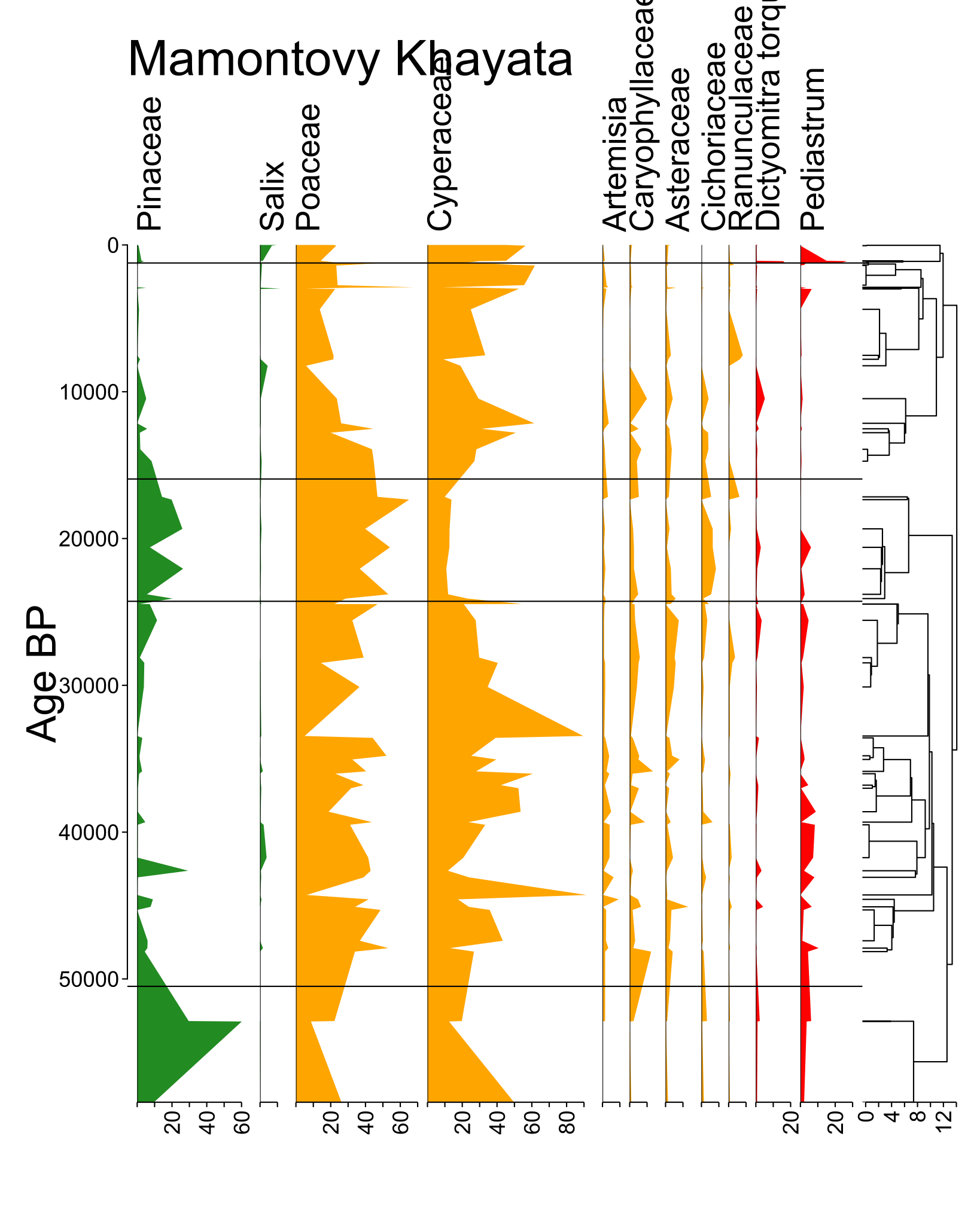
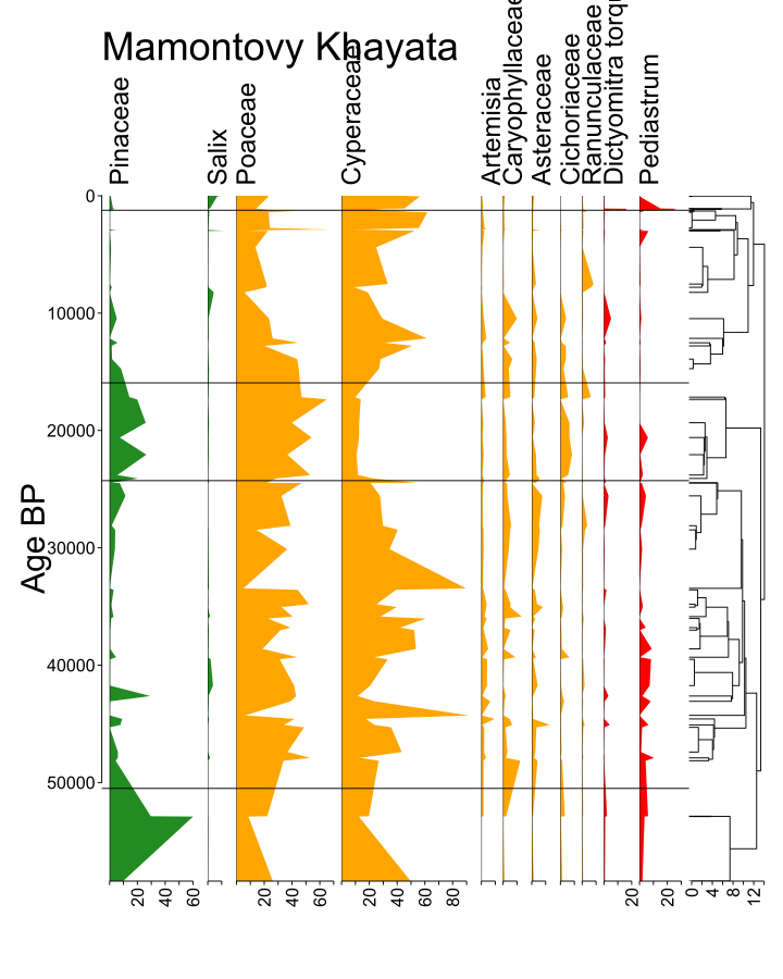
English: Pollen diagram of Mamontovy Khayata, North Siberia, Laptev sea coast, near eastern Lena river delta , near Tiksi and Bykovskiy |
| Date | |
| Source | Own work |
| Author | Merikanto |
| Camera location | | View this and other nearby images on: OpenStreetMap |
|---|
This pollen diagram is based on data in Pangaea,
https://doi.pangaea.de/10.1594/PANGAEA.728482
https://doi.pangaea.de/10.1594/PANGAEA.728482?format=textfile
Andreev, Andrei A; Schirrmeister, Lutz; Siegert, Christine; Bobrov, Anatoly A; Demske, Dieter; Seiffert, Maria; Hubberten, Hans-Wolfgang (2002): Fig. 3: Pollen and spore counts of the Mamontovy Khayata sequences. PANGAEA, https://doi.org/10.1594/PANGAEA.728482, In supplement to: Andreev, AA et al. (2002): Paleoenvironmental changes in northeastern Siberia during the Late Quaternary - evidence from pollen records of the Bykovsky Peninsula. Polarforschung, 70, 13-25, https://doi.org/10.2312/polarforschung.70.13
@incollection{andreev2002fpas,
author={Andrei A {Andreev} and Lutz {Schirrmeister} and Christine {Siegert} and Anatoly A {Bobrov} and Dieter {Demske} and Maria {Seiffert} and Hans-Wolfgang {Hubberten}},
title=Template:Fig. 3: Pollen and spore counts of the Mamontovy Khayata sequences,
year={2002},
doi={10.1594/PANGAEA.728482},
url={https://doi.org/10.1594/PANGAEA.728482},
note={In supplement to: Andreev, AA et al. (2002): Paleoenvironmental changes in northeastern Siberia during the Late Quaternary - evidence from pollen records of the Bykovsky Peninsula. Polarforschung, 70, 13-25, https://doi.org/10.2312/polarforschung.70.13},
type={data set},
publisher={PANGAEA}
}
"R" code to produce this pollen plot
- pollen diagram of Mamontovy Khayata
- 28.10.21 0000.0005
-
library("tidyverse")
library("dplyr")
library("stringi")
library("stringr")
library("pracma")
library("ggplot2")
library("cowplot")


library("neotoma")
library("rioja")
library("ggpalaeo") #Need new version
plot_taxons=1
plot_groups=0
plot_to_svg=1
- minimum pollen count %
minpercent1=40
sitename1="Mamontovy Khayata"
- from Pangaea
- https://doi.pangaea.de/10.1594/PANGAEA.728482
finame1<-"Mamontovy_Khayata_pollen_spores.tab"


sitename_x0=tolower(sitename1)
sitename_x1<-str_replace(sitename_x0,' ', '_')
outfilename1<-paste0("./",sitename_x1,"_pollen_n.svg")
outfilename2<-paste0("./",sitename_x1,"_pollen_groups_1.svg")


	#dev.off()


in1<- readLines(finame1)


length1<-length(in1)
- print (length1)
n=1
loc1=n
in_komments=0
in_species=0


long_specie_table_00<-vector()
for(n in 1:length1)
{
	rowi=in1[n]
	sica=substr(rowi,1,2)
	sica2=substr(rowi,1,13)
	sica3=substr(rowi,1,8)
	#print(sica)
	#print(n)
	if(in_species==1)
	{
			if (identical(sica3,"License:"))
			{
				sica3=""
				in_species=0
			}
	}


	if(in_species==1)
	{
		#print(rowi)
		specie01<-word(rowi,1,sep = "\\ \\[")
		specie02<-word(specie01,1,sep = "\\ \\*")
		#print(specie1)
		specie2<-sub("\t", "", specie02)
		long_specie_table_00<-c(long_specie_table_00, specie2)
		#print(specie2)
	}


	if(in_komments==1)
		{
		if (identical(sica2,"Parameter(s):"))
			{
				sica2=""
				in_species=1
				#print(rowi)
				#stop(-3)
			}
		}


	if (identical(sica,"/*"))
		{
			in_komments=1
			#"comment in"
			#break
		}
	if (identical(sica,"*/"))
		{
			in_komments=0
			in_species=0
			#"comment out"
			loc1=n
			break
		}
}
- stop(-4)
namef1<-read.csv(finame1, skip = loc1,nrows=1, sep="	",header = F)
dataf1 = read.csv(finame1, skip = loc1+1, sep="	",header = F)
- namef1
- dataf1
rowlen1<-nrow(dataf1)
collen1<-ncol(dataf1)
- print (collen1)
ages1<-dataf1["V1"]
ages1<-ages1*1000
poldatas1<-dataf1[5:57]
polnames1<-namef1[5:57]
groupdatas1<-dataf1[58:62]
groupnames1<-namef1[58:62]
long_specie_table_01<-long_specie_table_00[4:56]
- long_specie_table_01
long_polnames01<-as.data.frame(long_specie_table_01)
names(long_polnames01)<-"taxon"
long_polnames1=data.frame(t(long_polnames01))
- stop(-1)
names(ages1)<-"age"
names(polnames1)<-c("taxon")


polnames1 <- data.frame(lapply(polnames1, function(x) {
                 gsub("\\[#\\]", "", x)
             }))
groupnames1 <- data.frame(lapply(groupnames1, function(x) {
                 gsub("\\ \\[#\\]", "", x)
             }))
- print("Data ...")
- print (polnames1)
- str(polnames1)
- str(long_polnames1)
- polak1<-rbind(polnames1,poldatas1)
polak1<-poldatas1
- names(polak1)<-polnames1
names(polak1)<-long_polnames1
- stop(-6)
width1<-ncol(polak1)


polak2<-polak1 / rowSums(polak1) * 100


polak2<-polak2[, colSums(polak2 != 0) > minpercent1]
- polak2
- polak3<-c(ages1,polak2)
polak3<-polak2
polak3<-cbind(ages1,polak3)
- polak3
- stop(-1)
polak3_spp <- polak3 %>%
	select(-age,)
	# %>%
	#as.data.frame()
- polak3_spp <- polak3 %>%
- select(-age,) %>%
- as.data.frame(polak3_spp)
- stop(-1)
polak3_dist <- dist(sqrt(polak3_spp/100))#chord distance
- stop(-1)
clust <- chclust(polak3_dist, method = "coniss")
- str(clust)
- stop(-1)
- p.col <- c(rep("forestgreen", times=width1))
- colors by eco groups, must tune by hand
p.col <- c(
	rep("forestgreen", times=2),
	rep("orange", times=7),
	rep("red", times=2)
)
- ages1
- y.scale=seq(0,60000,1000)
- y.scale=1:60
ages2<-ages1$age
y.scale=as.vector(ages2)
y.labels=y.scale
- str(y.scale)
if(plot_taxons==1)
{
	print("Taxons ...")
	## set up mgp for layout
	if(plot_to_svg==1)
	{
		svg(filename=outfilename1, width=8, height=10, pointsize=16)
	}


	mgp <- c(3, 0.25, 0)
	par(tcl = -0.15, mgp = mgp)#shorter axis ticks - see ?par


	pol.plot <- strat.plot(
	title=sitename1,
	ylabel = "Age BP",
	polak2,
	yvar=y.scale,
	#y.tks=y.scale,
	cex.xlabel = 1.2,
	cex.ylabel = 1.5,
	mgp = mgp,
	y.rev=TRUE, plot.line=FALSE, plot.poly=TRUE, plot.bar=FALSE,
	col.poly=p.col,
	scale.percent=TRUE, xSpace=0.01,
	x.pc.lab=TRUE, x.pc.omit0=TRUE, las=2,
	xRight = 0.98, #right margin
	xLeft = 0.13, #left margin with space for 2nd axis
	yTop = 0.8, #top margin
	yBottom = 0.1, #bottom margin
	clust = clust
	)
	addClustZone(pol.plot, clust = clust, nZone = 5)


	if(plot_to_svg==1)
	{
		dev.off()
	}
	print(".")
}


if(plot_groups==1)
{
	print("Groups ...")


	if(plot_to_svg==1)
	{
		svg(filename=outfilename2, width=8, height=10, pointsize=16)
	}


	names(groupdatas1)<-"group"
	names(groupnames1)<-"groupnames"


	#stop(-1)


	agelen1<-nrow(ages1)
	groupslen1<-length(groupnames1)
	print(agelen1)
	print(groupslen1)
	ages20<-as.vector(ages1$age)
	ages21<-rep(ages20,groupslen1)
	ages22<- (matrix(ages21, nrow = groupslen1, byrow = TRUE))
	ages2<-as.vector(ages22)
	groups20<-as.matrix(groupdatas1)
	groups21<-t(groups20)
	#groups22<-pracma::fliplr(groups21)
	#groups22<-pracma::flipud(groups21)
	groups22<-groups21
	groups2<-as.vector(groups22)
	groupnames20<-as.vector(t(groupnames1))
	groupnames21<-rep(groupnames20,agelen1)
	groupnames2<-as.vector(as.matrix(groupnames21))
	test <- data.frame(age=ages2,pollen=groups2, type=groupnames2)
	str(test)


	colors1<- rev(c("green","orange","red", "yellow", "violet"))
	#ggplot(test, aes(fill=type, y=pollen, x=age) )+
	#geom_area()


	# stacked area chart
	gee1<-ggplot(test, aes(fill=type, y=pollen, x=age) ) +
		ggtitle(sitename1)+
		#theme_nothing()+
		#geom_area(position="fill", stat="identity")+
		geom_area()+
		theme(legend.position=c(.9,.75))+
	#	geom_area()+
		#geom_text(aes(y = type, label = pollen, group =type), color = "white") +
		scale_color_manual(values = colors1 )+
		scale_fill_manual(values = colors1 )+
		scale_x_reverse()+
		coord_flip()
	plot(gee1)
	if(plot_to_svg==1)
	{
		dev.off()
	}


	print(".")
}
- print (poldatas1)
- print(in1[loc1])
- in1
Licensing[edit]
- You are free:
- to share – to copy, distribute and transmit the work
- to remix – to adapt the work
- Under the following conditions:
- attribution – You must give appropriate credit, provide a link to the license, and indicate if changes were made. You may do so in any reasonable manner, but not in any way that suggests the licensor endorses you or your use.
- share alike – If you remix, transform, or build upon the material, you must distribute your contributions under the same or compatible license as the original.
File history
Click on a date/time to view the file as it appeared at that time.
| Date/Time | Thumbnail | Dimensions | User | Comment | |
|---|---|---|---|---|---|
| current | 12:09, 26 October 2021 | | 720 × 900 (129 KB) | Merikanto (talk | contribs) | Update |
| 11:43, 26 October 2021 |  | 720 × 900 (116 KB) | Merikanto (talk | contribs) | Update | |
| 08:01, 26 October 2021 |  | 720 × 900 (132 KB) | Merikanto (talk | contribs) | Uploaded own work with UploadWizard |
You cannot overwrite this file.
File usage on Commons
There are no pages that use this file.