File:Schemat FIR tradycyjny.svg
Jump to navigation
Jump to search

Size of this PNG preview of this SVG file: 523 × 156 pixels. Other resolutions: 320 × 95 pixels | 640 × 191 pixels | 1,024 × 305 pixels | 1,280 × 382 pixels | 2,560 × 764 pixels.
Original file (SVG file, nominally 523 × 156 pixels, file size: 24 KB)
Captions
Captions
Add a one-line explanation of what this file represents
Summary
[edit]
| Description |
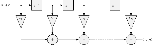
Polski: Tradycyjna struktura filtru SOI N-tego rzędu. Rysunek sporządzono na podstawie książki „Wprowadzenie do cyfrowego przetwarzania sygnałów” Richarda G. Lyonsa, s. 215. Zobacz też równoważną strukturę przekształconą tego filtru. |
| Date | |
| Source | Own work |
| Author | jdx |
| Other versions | |
| LaTeX source | click to expand
\documentclass[tikz]{standalone}

\usetikzlibrary{shapes.geometric, arrows}
\tikzstyle{dspsquare}=[rectangle, thick, draw=black, fill=gray!10, minimum size=1cm]
\tikzstyle{dspcircle}=[circle, thick, draw=black, fill=gray!10, minimum size=1cm]
\tikzstyle{dsptriangle}=[isosceles triangle, thick, draw=black, fill=gray!10, minimum size=1cm]
\tikzstyle{dspjoint}=[fill, draw=black, shape=circle, minimum size=3pt, inner sep=0]
\tikzstyle{dspio}=[draw=black, shape=circle, minimum size=5pt, inner sep=0]


\begin{document}

\begin{tikzpicture}[>=triangle 45]
\matrix(m1) [row sep=5mm, column sep=5mm]
{
    \node[dspio, label=left:$x(n)$]             (m00)   {};                     &
    \node[dspjoint]                             (m01)   {};                     &
    \node[dspsquare]                            (m02)   {$z^{-1}$};             &
    \node[dspjoint]                             (m03)   {};                     &
    \node[dspsquare]                            (m04)   {$z^{-1}$};             &
    \node[dspjoint]                             (m05)   {};                     &
    \node[inner sep=0]                          (m06)   {};                     &
    \node[inner sep=0]                          (m07)   {};                     &
    \node[dspsquare]                            (m08)   {$z^{-1}$};             &
    \node                                       (m09)   {};                     &
    \node                                       (m0a)   {};                     \\
    %------------------------------------------------------------------------------
    \node                                       (m10)   {};                     &
    \node[dsptriangle, shape border rotate=270] (m11)   {$b_0$};                &
    \node                                       (m12)   {};                     &
    \node[dsptriangle, shape border rotate=270] (m13)   {$b_1$};                &
    \node                                       (m14)   {};                     &
    \node[dsptriangle, shape border rotate=270] (m15)   {$b_2$};                &
    \node                                       (m16)   {};                     &
    \node                                       (m17)   {};                     &
    \node                                       (m18)   {};                     &
    \node[dsptriangle, shape border rotate=270] (m19)   {$b_N$};                &
    \node                                       (m1a)   {};                     \\
    %------------------------------------------------------------------------------
    \node                                       (m20)   {};                     &
    \node                                       (m21)   {};                     &
    \node                                       (m22)   {};                     &
    \node[dspcircle]                            (m23)   {$+$};                  &
    \node                                       (m24)   {};                     &
    \node[dspcircle]                            (m25)   {$+$};                  &
    \node[inner sep=0]                          (m26)   {};                     &
    \node[inner sep=0]                          (m27)   {};                     &
    \node[inner sep=0]                          (m28)   {};                     &
    \node[dspcircle]                            (m29)   {$+$};                  &
    \node[dspio, label=right:$y(n)$]            (m2a)   {};                     \\
    %------------------------------------------------------------------------------
};

\draw[->]   (m00) -- (m02);
\draw[->]   (m01) -- (m11);
\draw[->]   (m02) -- (m04);
\draw[->]   (m03) -- (m13);
\draw[-]    (m04) -- (m05);
\draw[->]   (m05) -- (m15);
\draw[-]    (m05) -- (m06);
\draw[-, densely dashed]   (m06) -- (m08);
\draw[->]   (m08) -| (m19);

\draw[->]   (m11) |- (m23);
\draw[->]   (m13) -- (m23);
\draw[->]   (m23) -- (m25);
\draw[->]   (m15) -- (m25);
\draw[-]    (m25) -- (m26);
\draw[-, densely dashed]   (m26) -- (m28);
\draw[->]   (m28) -- (m29);
\draw[->]   (m19) -- (m29);
\draw[-]    (m29) -- (m2a);
\end{tikzpicture}

\end{document}
|
W3C-validity not checked.
Licensing
[edit]
I, the copyright holder of this work, hereby publish it under the following license:
This file is licensed under the Creative Commons Attribution-Share Alike 3.0 Unported license.
- You are free:
- to share – to copy, distribute and transmit the work
- to remix – to adapt the work
- Under the following conditions:
- attribution – You must give appropriate credit, provide a link to the license, and indicate if changes were made. You may do so in any reasonable manner, but not in any way that suggests the licensor endorses you or your use.
- share alike – If you remix, transform, or build upon the material, you must distribute your contributions under the same or compatible license as the original.
File history
Click on a date/time to view the file as it appeared at that time.
| Date/Time | Thumbnail | Dimensions | User | Comment | |
|---|---|---|---|---|---|
| current | 16:36, 18 July 2015 | 523 × 156 (24 KB) | Jdx (talk | contribs) | {{Information |Description ={{pl|1=Tradycyjna struktura filtru SOI. Rysunek sporządzono na podstawie książki „Wprowadzenie do cyfrowego przetwarzania sygnałów” Richarda G. Lyonsa, s. 215. Zo... |
You cannot overwrite this file.
File usage on Commons
The following 2 pages use this file: