File:Butterworth response.png
原始檔案 (1,240 × 880 像素,檔案大小:86 KB,MIME 類型:image/png)
說明
說明
摘要
[編輯]| 描述 |
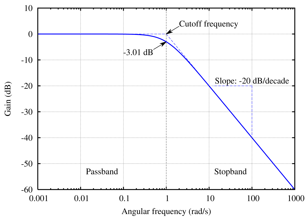
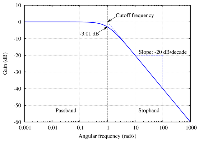
English: The frequency response of a Butterworth filter with logarithmic axes (Bode plot) and various labels. Cutoff frequency is normalized to 1 rad/s. Gain is normalized to 0 dB in the passband.
Many orders on one plot: File:Butterworth orders.png. Version with no text available at File:Butterworth plain.png, though you should probably just modify the source code and regenerate it in your own language. See Wikipedia graph-making tips. Generated in gnuplot with the script below (save as butterworth.plt and then open in gnuplot). Then I opened the butterworth.ps file in a text editor to edit the line colors and linestyles, as per this description. This avoids needing to open in proprietary software, and really isn't that difficult (especially if you don't know the commands in the proprietary software either). ;-) Identify the lines easily by their color (the arrow is currently magenta and I want it to be black. Ah, there is the entry with 1 0 1, red + blue = magenta) or by using the gnuplot linestyle−1. (For instance, gnuplot's linestyle 3 corresponds to the ps file's /LT2.) Then you can edit the colors and dashes by hand. I changed the original: /LT0 { PL [] 1 0 0 DL } def
/LT1 { PL [4 dl 2 dl] 0 1 0 DL } def
/LT2 { PL [2 dl 3 dl] 0 0 1 DL } def
/LT3 { PL [1 dl 1.5 dl] 1 0 1 DL } def
into this: /LT0 { PL [] 0 0 1 DL } def
/LT1 { PL [4 dl 2 dl] 0.5 0.5 0.5 DL } def
/LT2 { PL [6 dl 3 dl] 0.3 0.3 1 DL } def
/LT3 { PL [] 0 0 0 DL } def
/LT4–/LT8 I left unchanged. (I don't know what they're used for anyway.) /LTw, /LTb, and /LTa are for the grid lines and such.To convert the PostScript file to PNG:
|
| 日期 | 2005年六月26日 (上傳日期) |
| 來源 | 自己的作品 |
| 作者 | Omegatron |
| 其他版本 |
|
| gnuplot source | click to expand
set samples 2001
set terminal postscript enhanced landscape color lw 2 "Times-Roman" 20
set output "butterworth.ps"

# Butterworth amplitude response and decibel calculation.  n is the order, which is just 1 in this image.
G(w,n) = 1 / (sqrt(1 + w**(2*n)))
dB(x) = 20 * log10(abs(x))

# Gridlines
set grid

# Set x axis to logarithmic scale
set logscale x 10

# Set range of x and y axes
set xrange [0.001:1000]
set yrange [-60:10]

# Create x-axis tic marks once per decade (every multiple of 10)
set xtics 10

# Use 10 x-axis minor divisions per major division
set mxtics 10

# Axis labels
set xlabel "Angular frequency (rad/s)"
set ylabel "Gain (dB)"

# No need for a key
set nokey #0.1,-25

# Frequency response's line plotting style
set style line 1 lt 1 lw 2

# Draw a separator between passband and stopband and label them
set style line 2 lt 2 lw 1
set style arrow 2 nohead ls 2
set arrow 3 from 1,-60 to 1,10 as 2

# Label coordinates are relative to the graph window, not to the function, centered at the 1/4 and 3/4 width points
set label 1 "Passband" at graph 0.25, graph 0.1 c
set label 2 "Stopband" at graph 0.75, graph 0.1 c

# Asymptote lines and slope lines are the same "arrow" style
set style line 3 lt 3 lw 1
set style arrow 3 nohead ls 3

# Draw asymptote lines
set arrow 1 from 1,0 to 1000,-60 as 3
set arrow 2 from .001,0 to 1,0 as 3

# -3 dB arrow style and arrow
set style line 4 lt 4 lw 1
set style arrow 4 head filled size screen 0.02,15,45 ls 4
set arrow 4 from 2,3 to 1,0 as 4

# "Cutoff frequency" label uses same coordinates as the function
set label 3 "Cutoff frequency" at 2,4 l

# "-3 dB" label
set arrow 5 from 0.5,-6 to 1,-3 as 4
set label 4 "-3.01 dB" at 0.5,-7 r

# Draw slope lines and label
set arrow 6 from 100,-20 to 12,-20 as 3
set arrow 7 from 100,-20 to 100,-39 as 3
set label 5 "Slope: -20 dB/decade" at 100,-18 c

# Plot the filter response
plot \
     dB(G(x,1)) ls 1  title "1st-order response"
|


|
File:Butterworth response.svg是本檔案的向量版本。 如果品質不低,就應該優先使用該檔案,而非PNG檔案。
File:Butterworth response.png → File:Butterworth response.svg
更多資訊請參閱Help:SVG/zh。 |
 |
授權條款
[編輯]

|
已授權您依據自由軟體基金會發行的無固定段落、封面文字和封底文字GNU自由文件授權條款1.2版或任意後續版本,對本檔進行複製、傳播和/或修改。該協議的副本列在GNU自由文件授權條款中。 |
檔案歷史
點選日期/時間以檢視該時間的檔案版本。
| 日期/時間 | 縮圖 | 尺寸 | 用戶 | 備註 | |
|---|---|---|---|---|---|
| 目前 | 2005年7月23日 (六) 17:45 | | 1,240 × 880(86 KB) | Omegatron(對話 | 貢獻) | split the cutoff frequency markers |
| 2005年7月23日 (六) 16:31 |  | 1,250 × 880(92 KB) | Omegatron(對話 | 貢獻) | Better butterworth filter response curve | |
| 2005年6月26日 (日) 19:54 |  | 250 × 220(2 KB) | Omegatron(對話 | 貢獻) | A graph or diagram made by User:Omegatron. (Uploaded with Wikimedia Commons.) Source: Created by User:Omegatron {{GFDL}}{{cc-by-sa-2.0}} Category:Diagrams\ |
無法覆蓋此檔案。
檔案用途
下列5個頁面有用到此檔案:
全域檔案使用狀況
以下其他 wiki 使用了這個檔案:
- be-tarask.wikipedia.org 的使用狀況
- de.wikipedia.org 的使用狀況
- eo.wikipedia.org 的使用狀況
- et.wikipedia.org 的使用狀況
- fr.wikipedia.org 的使用狀況
- hi.wikipedia.org 的使用狀況
- it.wikipedia.org 的使用狀況
- ja.wikipedia.org 的使用狀況
- pl.wikipedia.org 的使用狀況
- pt.wikipedia.org 的使用狀況
- zh.wikipedia.org 的使用狀況