File:MUSIC MVDR.png
Salta a la navegació
Salta a la cerca

Mida d'aquesta previsualització: 800 × 386 píxels. Altres resolucions: 320 × 154 píxels | 640 × 309 píxels | 1.342 × 647 píxels.
Fitxer original (1.342 × 647 píxels, mida del fitxer: 112 Ko, tipus MIME: image/png)
Llegendes
Llegendes
Afegeix una explicació d'una línia del que representa aquest fitxer
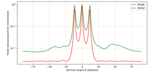
The frequency estimation based on MUSIC and MVDR algorithms.
Resum
[modifica]
| Descripció |
English: Spatial frequencies estimation (source code).
Русский: Оценка пространтвенных частот (исходный код). |
| Data | |
| Font | Treball propi |
| Autor | Kirlf |
| PNG genesis | Aquesta PNG imatge rasteritzada ha estat creada amb Matplotlib |
| Codi font | Python code"""
Developed by Vladimir Fadeev
(https://github.com/kirlf)
Kazan, 2017 / 2020
Python 3.7
"""
import numpy as np
import matplotlib.pyplot as plt
"""
Received signal model:
X = A*S + W
where
A = [a(theta_1) a(theta_2) ... a(theta_d)]
is the matrix of steering vectors
(dimension is M x d,
M is the number of sensors,
d is the number of signal sources),
A steering vector represents the set of phase delays
a plane wave experiences, evaluated at a set of array elements (antennas).
The phases are specified with respect to an arbitrary origin.
theta is Direction of Arrival (DoA),
S = 1/sqrt(2) * (X + iY)
is the transmit (modulation) symbols matrix
(dimension is d x T,
T is the number of snapshots)
(X + iY) is the complex values of the signal envelope,
W = sqrt(N0/2)*(G1 + jG2)
is additive noise matrix (AWGN)
(dimension is M x T),
N0 is the noise spectral density,
G1 and G2 are the random Gaussian distributed values.
"""
M = 10 # number of sensors
SNR = 10 # Signal-to-Noise ratio (dB)
d = 3 # number sources of EM waves
N = 50 # number of snapshots
""" Signal matrix """
S = ( np.sign(np.random.randn(d,N)) + 1j * np.sign(np.random.randn(d,N)) ) / np.sqrt(2) # QPSK
""" Noise matrix
Common formula:
AWGN = sqrt(N0/2)*(G1 + jG2),
where G1 and G2 - independent Gaussian processes.
Since Es(symbol energy) for QPSK is 1 W, noise spectral density:
N0 = (Es/N)^(-1) = SNR^(-1) [W] (let SNR = Es/N0);
or in logarithmic scale::
SNR_dB = 10log10(SNR) -> N0_dB = -10log10(SNR) = -SNR_dB [dB];
We have SNR in logarithmic (in dBs), convert to linear:
SNR = 10^(SNR_dB/10) -> sqrt(N0) = (10^(-SNR_dB/10))^(1/2) = 10^(-SNR_dB/20)
"""
W = ( np.random.randn(M,N) + 1j * np.random.randn(M,N) ) / np.sqrt(2) * 10**(-SNR/20) # AWGN
mu_R = 2*np.pi / M # standard beam width
resolution_cases = ((-1., 0, 1.), (-0.5, 0, 0.5), (-0.3, 0, 0.3)) # resolutions
for idxm, c in enumerate(resolution_cases):
""" DoA (spatial frequencies) """
mu_1 = c[0]*mu_R
mu_2 = c[1]*mu_R
mu_3 = c[2]*mu_R
""" Steering vectors """
a_1 = np.exp(1j*mu_1*np.arange(M))
a_2 = np.exp(1j*mu_2*np.arange(M))
a_3 = np.exp(1j*mu_3*np.arange(M))
A = (np.array([a_1, a_2, a_3])).T # steering matrix
""" Received signal """
X = np.dot(A,S) + W
""" Rxx """
R = np.dot(X,np.matrix(X).H)
U, Sigma, Vh = np.linalg.svd(X, full_matrices=True)
U_0 = U[:,d:] # noise sub-space
thetas = np.arange(-90,91)*(np.pi/180) # azimuths
mus = np.pi*np.sin(thetas) # spatial frequencies
a = np.empty((M, len(thetas)), dtype = complex)
for idx, mu in enumerate(mus):
a[:,idx] = np.exp(1j*mu*np.arange(M))
# MVDR:
S_MVDR = np.empty(len(thetas), dtype = complex)
for idx in range(np.shape(a)[1]):
a_idx = (a[:, idx]).reshape((M, 1))
S_MVDR[idx] = 1 / (np.dot(np.matrix(a_idx).H, np.dot(np.linalg.pinv(R),a_idx)))
# MUSIC:
S_MUSIC = np.empty(len(thetas), dtype = complex)
for idx in range(np.shape(a)[1]):
a_idx = (a[:, idx]).reshape((M, 1))
S_MUSIC[idx] = np.dot(np.matrix(a_idx).H,a_idx)\
/ (np.dot(np.matrix(a_idx).H, np.dot(U_0,np.dot(np.matrix(U_0).H,a_idx))))
plt.subplots(figsize=(10, 5), dpi=150)
plt.semilogy(thetas*(180/np.pi), np.real( (S_MVDR / max(S_MVDR))), color='green', label='MVDR')
plt.semilogy(thetas*(180/np.pi), np.real((S_MUSIC/ max(S_MUSIC))), color='red', label='MUSIC')
plt.grid(color='r', linestyle='-', linewidth=0.2)
plt.xlabel('Azimuth angles (degrees)')
plt.ylabel('Power (pseudo)spectrum (normalized)')
plt.legend()
plt.title('Case #'+str(idxm+1))
plt.show()
""" References
1. Haykin, Simon, and KJ Ray Liu. Handbook on array processing and sensor networks. Vol. 63. John Wiley & Sons, 2010. pp. 102-107
2. Hayes M. H. Statistical digital signal processing and modeling. – John Wiley & Sons, 2009.
3. Haykin, Simon S. Adaptive filter theory. Pearson Education India, 2008. pp. 422-427
4. Richmond, Christ D. "Capon algorithm mean-squared error threshold SNR prediction and probability of resolution." IEEE Transactions on Signal Processing 53.8 (2005): 2748-2764.
5. S. K. P. Gupta, MUSIC and improved MUSIC algorithm to esimate dorection of arrival, IEEE, 2015.
"""
|
Llicència
[modifica]
Jo, el titular dels drets d'autor d'aquest treball, el public sota la següent llicència:
This file is licensed under the Creative Commons Attribution-Share Alike 4.0 International license.
- Sou lliure de:
- compartir – copiar, distribuir i comunicar públicament l'obra
- adaptar – fer-ne obres derivades
- Amb les condicions següents:
- reconeixement – Heu de donar la informació adequada sobre l'autor, proporcionar un enllaç a la llicència i indicar si s'han realitzat canvis. Podeu fer-ho amb qualsevol mitjà raonable, però de cap manera no suggereixi que l'autor us dóna suport o aprova l'ús que en feu.
- compartir igual – Si modifiqueu, transformeu, o generareu amb el material, haureu de distribuir les vostres contribucions sota una llicència similar o una de compatible com l'original
Historial del fitxer
Cliqueu una data/hora per veure el fitxer tal com era aleshores.
| Data/hora | Miniatura | Dimensions | Usuari/a | Comentari | |
|---|---|---|---|---|---|
| actual | 05:41, 18 feb 2019 | | 1.342 × 647 (112 Ko) | Kirlf (discussió | contribucions) | User created page with UploadWizard |
No podeu sobreescriure aquest fitxer.
Ús del fitxer
No hi ha pàgines que utilitzin aquest fitxer.
Ús global del fitxer
Utilització d'aquest fitxer en altres wikis:
- Utilització a ca.wikipedia.org
- Utilització a en.wikipedia.org
- Utilització a ru.wikipedia.org
- Utilització a uk.wikipedia.org