File:Heteroclinic orbit in pendulum phaseportrait.png
Vai alla navigazione
Vai alla ricerca

Dimensioni di questa anteprima: 800 × 416 pixel. Altre risoluzioni: 320 × 166 pixel | 640 × 333 pixel | 1 017 × 529 pixel.
File originale (1 017 × 529 pixel, dimensione del file: 15 KB, tipo MIME: image/png)
Didascalie
Didascalie
Aggiungi una brevissima spiegazione di ciò che questo file rappresenta
Dettagli
[modifica]
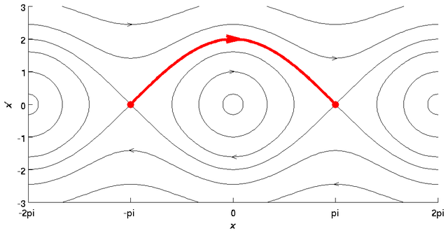
| Descrizione | Phaseportrait for the pendulum equation with the heteroclinic orbit highlighted. Created by Jitse Niesen using Matlab. |
| Data | 29 giugno 2006 (data di caricamento originaria) |
| Fonte | Nessuna fonte leggibile automaticamente. Presunta opera propria (secondo quanto affermano i diritti d'autore). |
| Autore | Nessun autore leggibile automaticamente. Jitse Niesen presunto (secondo quanto affermano i diritti d'autore). |
Discussion
[modifica]
How come the orbit isn't called homoclinic? The domain is periodic: starting and ending point are the same.
- That depends on what you consider as the domain. If the domain is a circle (and hence periodic), which is the most natural choice, then you're right and the orbit is homoclinic. If the domain is R, the set of real numbers, then the starting and ending point are not the same. But you certainly have a point that this is a confusing example; thanks for that. -- Jitse Niesen 06:45, 2 February 2007 (UTC)
Licenza
[modifica]
| Io, detentore del copyright su quest'opera, la rilascio nel pubblico dominio. Questa norma si applica in tutto il mondo. In alcuni paesi questo potrebbe non essere legalmente possibile. In tal caso: Garantisco a chiunque il diritto di utilizzare quest'opera per qualsiasi scopo, senza alcuna condizione, a meno che tali condizioni siano richieste dalla legge. |
Matlab source
[modifica]
clf;
axis([-2*pi 2*pi -3 3]);
daspect([1 1 1]);
hold on;

% Draw constant energy contours
qs = linspace(-2*pi, 2*pi, 101);
[Q,P] = meshgrid(qs, linspace(-3,3));
H = P.*P/2 - cos(Q);
contour(Q,P,H, [-0.95 -0.5 0.3  2 4], 'k');

% Draw energy = 0 contour
ps = sqrt(2+2*cos(qs));
plot(qs,ps, 'k');
plot(qs,-ps, 'k');

% Draw heteroclinic connection
qs = linspace(-pi, pi, 101);
ps = sqrt(2+2*cos(qs));
plot(qs,ps, 'r', 'LineWidth', 3);
plot([-pi pi], [0 0], 'r.', 'MarkerSize', 25);

% Arrows
plot(-pi+[-0.10 0.05], sqrt(6)+[0.05 0], 'k');
plot(-pi+[-0.10 0.05], sqrt(6)+[-0.05 0], 'k');
plot(pi+[-0.10 0.05], sqrt(2)+[0.05 0], 'k');
plot(pi+[-0.10 0.05], sqrt(2)+[-0.05 0], 'k');
plot([-0.10 0.05], [1.05 1], 'k');
plot([-0.10 0.05], [0.95 1], 'k');
plot([0.10 -0.05], -sqrt(2.6)+[0.05 0], 'k');
plot([0.10 -0.05], -sqrt(2.6)+[-0.05 0], 'k');
plot(-pi+[0.10 -0.05], -sqrt(2)+[0.05 0], 'k');
plot(-pi+[0.10 -0.05], -sqrt(2)+[-0.05 0], 'k');
plot(pi+[0.10 -0.05], -sqrt(6)+[0.05 0], 'k');
plot(pi+[0.10 -0.05], -sqrt(6)+[-0.05 0], 'k');
plot([-0.2 0.2], [2.1 2], 'r', 'LineWidth', 3);
plot([-0.2 0.2], [1.9 2], 'r', 'LineWidth', 3);

% Axes
xlabel('\it{x}');
ylabel('\it{x}''');
set(gca, 'XTick', [-2*pi -pi 0 pi 2*pi]);
set(gca, 'XTickLabel', {'-2pi' '-pi' '0' 'pi' '2pi'});

% Print
print -dpng 'heteroclinic_tmp.png';
system('convert -trim -bordercolor white -border 10 +repage heteroclinic_tmp.png heteroclinic.png');
Cronologia del file
Fare clic su un gruppo data/ora per vedere il file come si presentava nel momento indicato.
| Data/Ora | Miniatura | Dimensioni | Utente | Commento | |
|---|---|---|---|---|---|
| attuale | 10:50, 29 giu 2006 | | 1 017 × 529 (15 KB) | Jitse Niesen (discussione | contributi) | Phaseportrait for the pendulum equation with the heteroclinic orbit highlighted. Created by ~~~ using Matlab. |
Impossibile sovrascrivere questo file.
Utilizzo del file
Nessuna pagina utilizza questo file.
Utilizzo globale del file
Anche i seguenti wiki usano questo file:
- Usato nelle seguenti pagine di de.wikipedia.org:
- Usato nelle seguenti pagine di en.wikipedia.org:
- Usato nelle seguenti pagine di en.wikibooks.org:
- Usato nelle seguenti pagine di eo.wikipedia.org:
- Usato nelle seguenti pagine di it.wikipedia.org:
- Usato nelle seguenti pagine di ja.wikipedia.org: