File:Effect of circular convolution on discrete Hilbert transform.png
跳转到导航
跳转到搜索

本预览的尺寸:800 × 421像素。 其他分辨率:320 × 168像素 | 640 × 337像素 | 1,156 × 608像素。
原始文件 (1,156 × 608像素,文件大小:100 KB,MIME类型:image/png)
说明
说明
添加一行文字以描述该文件所表现的内容
摘要
[编辑]
| 描述 |
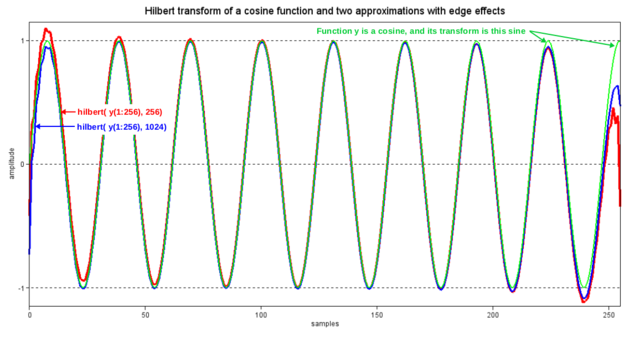
English: The Hilbert transform of cos(ωt) is sin(ωt). When a finite segment of cos(ωt) is transformed, edge effects inevitably occur. Using a segment length of 256 samples, this figure shows a sine function and two approximate Hilbert transforms computed by the MATLAB library function, hilbert(·), which supports optional zero-filling of the segment to be transformed. The red graph is the result of no zero-filling, and the blue graph is the result of 300% zero-filling. In the latter case, the edge effects are almost all due to the rise and fall times of the Hilbert transform's 2/(πn) impulse response. In the "red" case, we have the added effect of circular convolution. In other words, in the blue case, distortion occurs when some of the filter taps are coinciding with zeros, instead of with samples of cos(ωt). And in the red case, those same taps are coinciding with wrapped-around (and out-of-phase) samples of cos(ωt). |
|||
| 日期 | ||||
| 来源 | 自己的作品 | |||
| 作者 | Bob K | |||
| 授权 (二次使用本文件) |
我,本作品著作权人,特此采用以下许可协议发表本作品:
|
|||
| PNG开发 | 本PNG 位图使用LibreOffice创作。 |
|||
| Source file | Scilab codeN=256;
x=0:N-1;
cycles_per_segment = 8.2888; // empirical value that displays edge effects well
cycles_per_sample = cycles_per_segment/N;
Yreal = cos(2*%pi*cycles_per_sample*x); // function to be transformed
Ans = sin(2*%pi*cycles_per_sample*x); // the ideal answer
H1 = imag(hilbert(Yreal)); // no zero-filling
H2 = imag(hilbert([Yreal zeros(1,1024-N)])); // zero-filling
// Display the results
red=5; blue=2; green=3; black=1; // based on a call to getcolor()
top=green; middle=blue; bottom=red;
plot2d(x', [H1' H2(1:N)' Ans'], style=[bottom middle top], rect=[0,-1.15,N-1,1.15]);
a = gca();
a.box = "on";
a.font_size=2; //set the tics label font size
a.visible = "on";
a.grid = [-1,0];
a.auto_ticks = ["off","off","off"]
a.y_ticks = tlist(["ticks", "locations", "labels"], [-1 0 1], ["-1" "0" "1"]);
a.x_ticks = tlist(["ticks", "locations", "labels"], [0 50 100 150 200 250], ["0" "50" "100" "150" "200" "250"]);
//a.children.children.thickness=2; // set line thickness of plots
top=1; middle=2; bottom=3;
a.children.children(top).thickness=2;
a.children.children(middle).thickness=3;
a.children.children(bottom).thickness=4;
xlabel("samples", "fontsize", 2)
ylabel("amplitude", "fontsize", 2)
title("Hilbert transform of a cosine function and two approximations with edge effects", "fontsize", 4)
|
See also
[编辑]
文件历史
点击某个日期/时间查看对应时刻的文件。
| 日期/时间 | 缩略图 | 大小 | 用户 | 备注 | |
|---|---|---|---|---|---|
| 当前 | 2016年2月9日 (二) 10:58 | | 1,156 × 608(100 KB) | Bob K(留言 | 贡献) | Show the sine function and 2 approximations, instead of the 2 difference functions. |
| 2015年4月10日 (五) 15:34 |  | 1,083 × 570(23 KB) | Bob K(留言 | 贡献) | The new figure compares two different error functions, one with zero-filling and one without. | |
| 2012年9月14日 (五) 01:26 |  | 1,139 × 636(9 KB) | Bob K(留言 | 贡献) | shift horizontal scale by 1 | |
| 2012年9月14日 (五) 00:48 |  | 1,134 × 632(9 KB) | Bob K(留言 | 贡献) | Larger font size for labels | |
| 2012年9月13日 (四) 22:51 |  | 1,119 × 610(7 KB) | Bob K(留言 | 贡献) | User created page with UploadWizard |
您不可以覆盖此文件。
文件用途
以下4个页面使用本文件:
全域文件用途
以下其他wiki使用此文件:
- en.wikipedia.org上的用途
- ko.wikipedia.org上的用途
- zh.wikipedia.org上的用途