File:Plot of x^y = y^x.png
From Wikimedia Commons, the free media repository
Jump to navigation
Jump to search

Size of this preview: 588 × 599 pixels. Other resolutions: 236 × 240 pixels | 471 × 480 pixels | 688 × 701 pixels.
Original file (688 × 701 pixels, file size: 46 KB, MIME type: image/png)
File information
Structured data
Captions
Captions
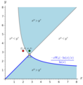
Plot of equation x^y = y^x with inequility regions highlighted.
Summary[edit]
| DescriptionPlot of x^y = y^x.png |
English: The boundary of the blue and white regions are the points where  . The blue region corresponds to . The blue region corresponds to  and the white region corresponds to and the white region corresponds to  . The bottom blue curve can be written explicitly by the expression . The bottom blue curve can be written explicitly by the expression  , where , where  is the Lambert W function. The top green curve is is the Lambert W function. The top green curve is  , and the gray curve is , and the gray curve is  . From the plot, we can see that . From the plot, we can see that  and and  . . |
||
| Date | |||
| Source | Own work | ||
| Author | Hugo Spinelli | ||
| Other versions | Plot of x^y = y^x.svg | ||
| Source code InfoField | Try it here (permalink).
|
Licensing[edit]
I, the copyright holder of this work, hereby publish it under the following license:
| This file is made available under the Creative Commons CC0 1.0 Universal Public Domain Dedication. | |
| The person who associated a work with this deed has dedicated the work to the public domain by waiving all of their rights to the work worldwide under copyright law, including all related and neighboring rights, to the extent allowed by law. You can copy, modify, distribute and perform the work, even for commercial purposes, all without asking permission.
http://creativecommons.org/publicdomain/zero/1.0/deed.enCC0Creative Commons Zero, Public Domain Dedicationfalsefalse |
File history
Click on a date/time to view the file as it appeared at that time.
| Date/Time | Thumbnail | Dimensions | User | Comment | |
|---|---|---|---|---|---|
| current | 04:11, 26 September 2023 |  | 688 × 701 (46 KB) | Hugo Spinelli (talk | contribs) | Added expressions for the other boundary curves. |
| 03:48, 26 September 2023 |  | 688 × 701 (39 KB) | Hugo Spinelli (talk | contribs) | Uploaded own work with UploadWizard |
You cannot overwrite this file.
File usage on Commons
There are no pages that use this file.
Metadata
This file contains additional information such as Exif metadata which may have been added by the digital camera, scanner, or software program used to create or digitize it. If the file has been modified from its original state, some details such as the timestamp may not fully reflect those of the original file. The timestamp is only as accurate as the clock in the camera, and it may be completely wrong.
| Software used | |
|---|---|
| Horizontal resolution | 59.06 dpc |
| Vertical resolution | 59.06 dpc |
Structured data
Items portrayed in this file
depicts
image/png
62f8e5635a792dc7e2a13c32878952c8ede4939d
46,925 byte
701 pixel
688 pixel
Hidden categories: