File:Butterworth filter bode plot.svg

原始檔案 (SVG 檔案,表面大小:1,250 × 875 像素,檔案大小:31 KB)
說明
說明
摘要
[編輯]| 描述 |
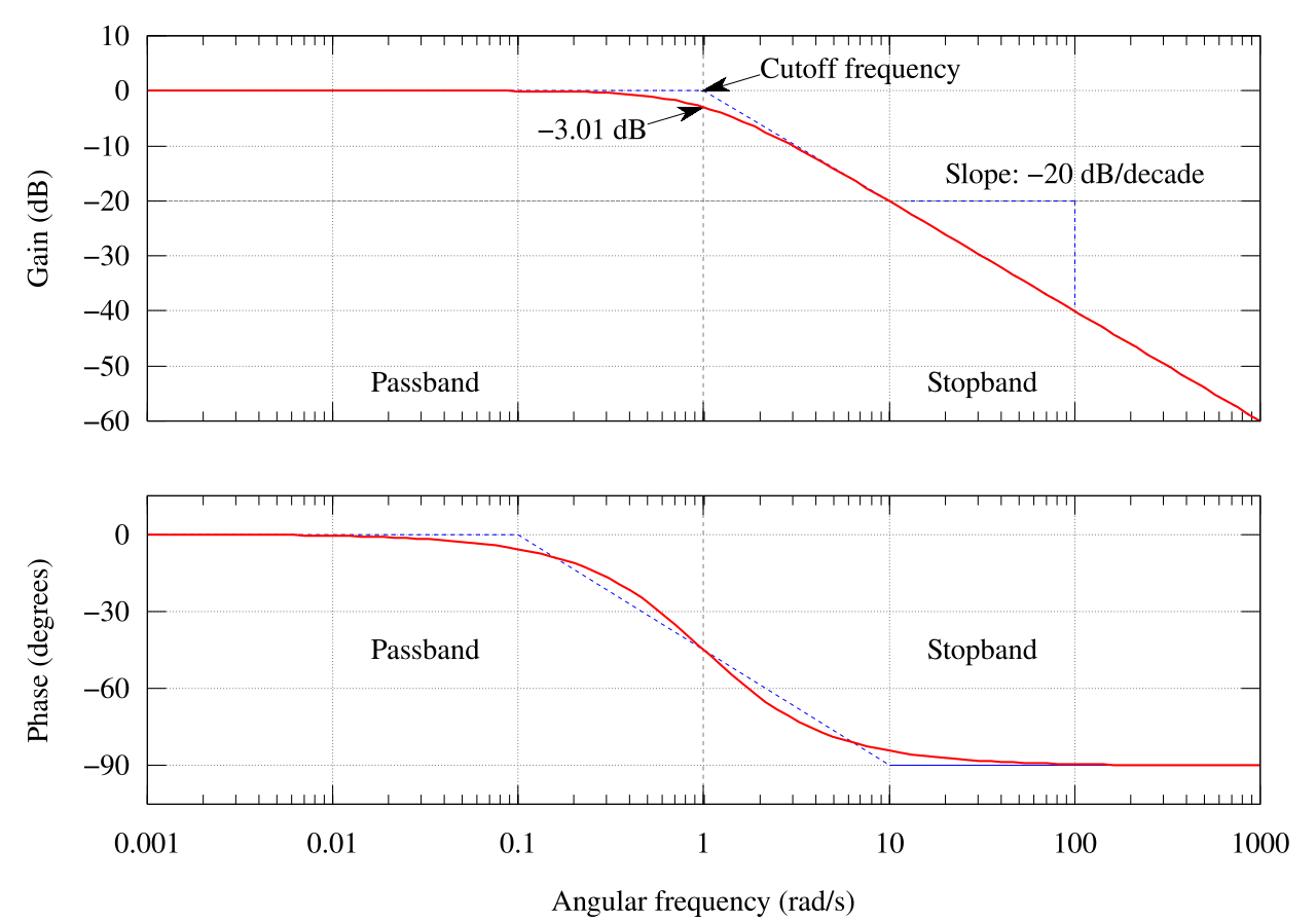
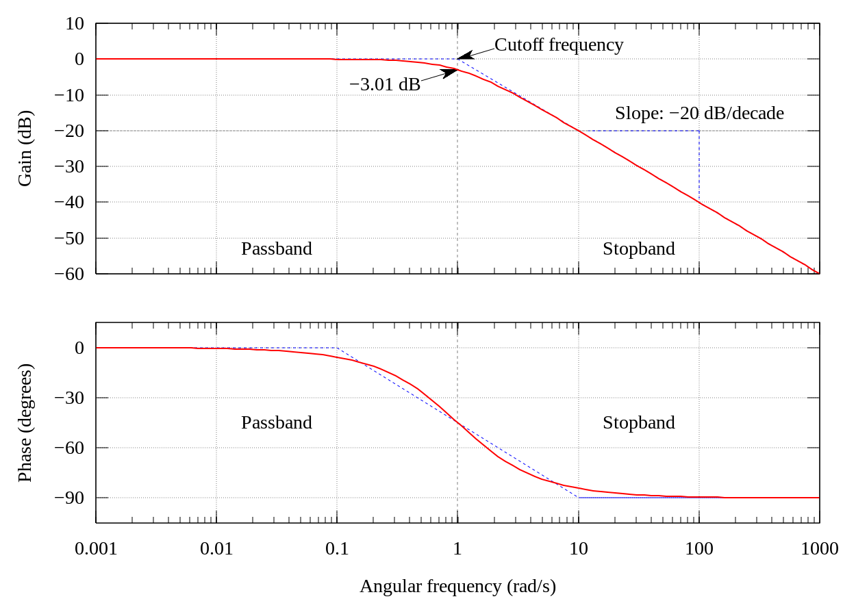
English: The Bode plot of a Butterworth filter with logarithmic axes and various labels. Cutoff frequency is normalized to 1 rad/s. Gain is normalized to 0 dB in the passband. Phase is in degrees because that's typical.
The code is kind of kludgy, but makes a good output. Generated in gnuplot with the script below (save as butterworth_bode_plot.plt and then open in gnuplot). Then it was postprocessed with Inkscape. See Wikipedia graph-making tips. Many orders on one plot: Image:Butterworth orders.png
本vector image使用Gnuplot創作。 |
||
| 日期 | 2006年4月26日 (上傳日期) | ||
| 來源 | 自己的作品 | ||
| 作者 | Alejo2083 | ||
| 其他版本 |
[]
.png:
|
||
| gnuplot source | click to expand
set terminal svg enhanced size 1250 875 fname "Times" fsize 25
set output "Butterworth_filter_bode_plot.svg"

# Butterworth amplitude response and decibel calculation.  n is the order, which is just 1 in this image.
G(w,n) = 1 / (sqrt(1 + w**(2*n)))
dB(x) = 20 * log10(abs(x))
# Phase is for first order
P(w) = -atan(w)*180/pi


# Gridlines
set grid

# Set x axis to logarithmic scale
set logscale x 10

# No need for a key
set nokey #0.1,-25

# Frequency response's line plotting style
set style line 1 lt 1 lw 2

# Asymptote lines and slope lines are the same "arrow" style
set style line 3 lt 3 lw 1
set style arrow 3 nohead ls 3

# -3 dB arrow style
set style line 4 lt 4 lw 1
set style arrow 4 head filled size screen 0.02,15,45 ls 4

# Separator between passband and stopband line style
set style line 2 lt 2 lw 1
set style arrow 2 nohead ls 2


set multiplot

# Magnitude response
# =============================================
set size 1,0.5
set origin 0,0.5

# Set range of x and y axes
set xrange [0.001:1000]
set yrange [-60:10]

# Create x-axis tic marks once per decade (every multiple of 10)
set xtics 10
#set ytics 10

# No need for two sets of numbers
set format x ""

# Use 10 x-axis minor divisions per major division
set mxtics 10

# Axis labels
set ylabel "Gain (dB)"

# Draw asymptote lines
set arrow 1 from 1,0 to 1000,-60 as 3
set arrow 2 from .001,0 to 1,0 as 3

# -3 dB arrow
set arrow 4 from 2,3 to 1,0 as 4

# "Cutoff frequency" label uses same coordinates as the function
set label 3 "Cutoff frequency" at 2,4 l

# "-3 dB" label
set arrow 5 from 0.5,-6 to 1,-3 as 4
set label 4 "-3.01 dB" at 0.5,-7 r

# Draw a separator between passband and stopband and label them
set arrow 3 from 1,-60 to 1,10 as 2

# Label coordinates are relative to the graph window, not to the function, centered at the 1/4 and 3/4 width points
set label 1 "Passband" at graph 0.25, graph 0.1 c
set label 2 "Stopband" at graph 0.75, graph 0.1 c

# Draw slope lines and label
set arrow 6 from 100,-20 to 12,-20 as 3
set arrow 7 from 100,-20 to 100,-39 as 3
set label 5 "Slope: -20 dB/decade" at 100,-15 c

plot dB(G(x,1)) ls 1  title "1st-order response"


#Phase response
# =============================================
set size 1,0.5
set origin 0,0

# Set range of x and y axes
set yrange [-105:15]

# Create y-axis tic marks every 15 degrees
set ytics 30

# Regular numbers
set format x "% g"

# Axis labels
set ylabel "Phase (degrees)"
set xlabel "Angular frequency (rad/s)"

# Draw asymptote lines
set arrow 1 from 0.1,0 to 10,-90 as 3
set arrow 2 from 0.001,0 to 0.1,0 as 3
set arrow 10 from 10,-90 to 1000,-90 as 3

# -3 dB arrow
unset arrow 4 #from 2,3 to 1,0 as 4

# "Cutoff frequency" label uses same coordinates as the function
unset label 3 #"Cutoff frequency" at 2,4 l

# "-3 dB" label
unset arrow 5 #from 0.5,-6 to 1,-3 as 4
unset label 4 #"-3.01 dB" at 0.5,-7 r

# Draw a separator between passband and stopband and label them
set arrow 3 from 1,-105 to 1,15 as 2

# Label coordinates are relative to the graph window, not to the function, centered at the 1/4 and 3/4 width points
set label 1 "Passband" at graph 0.25, graph 0.5 c
set label 2 "Stopband" at graph 0.75, graph 0.5 c

# Draw slope lines and label
unset arrow 6 #from 100,-20 to 12,-20 as 3
unset arrow 7 #from 100,-20 to 100,-39 as 3
unset label 5 #"Slope: -20 dB/decade" at 100,-18 c

plot P(x) ls 1 title "Phase response"


unset multiplot
|


|
本圖像有可用的柵格版本。當其品質較佳時,就應該替代此矢量圖像。
File:Butterworth filter bode plot.svg → File:Butterworth filter bode plot.png
通常,最好使用好的矢量版本(SVG)。 |
 |
授權條款
[編輯]

|
已授權您依據自由軟體基金會發行的無固定段落、封面文字和封底文字GNU自由文件授權條款1.2版或任意後續版本,對本檔進行複製、傳播和/或修改。該協議的副本列在GNU自由文件授權條款中。 |
| 此檔案採用創用CC 姓名標示-相同方式分享 3.0 未在地化版本授權條款。 | ||
| ||
| 已新增授權條款標題至此檔案,作為GFDL授權更新的一部份。 |
檔案歷史
點選日期/時間以檢視該時間的檔案版本。
| 日期/時間 | 縮圖 | 尺寸 | 使用者 | 備註 | |
|---|---|---|---|---|---|
| 目前 | 2023年10月12日 (四) 02:39 | | 1,250 × 875(31 KB) | Mikhail Ryazanov(留言 | 貢獻) | +ru translation |
| 2023年10月12日 (四) 02:19 |  | 1,250 × 875(30 KB) | Mikhail Ryazanov(留言 | 貢獻) | trying Glrx's advice | |
| 2023年10月12日 (四) 02:01 |  | 1,250 × 875(30 KB) | Glrx(留言 | 貢獻) | try fixing two -30 labels // Editing SVG source code using c:User:Rillke/SVGedit.js | |
| 2023年10月11日 (三) 23:46 |  | 1,250 × 875(30 KB) | Mikhail Ryazanov(留言 | 貢獻) | wrong rendering | |
| 2023年10月11日 (三) 23:45 |  | 1,250 × 875(30 KB) | Mikhail Ryazanov(留言 | 貢獻) | hyphens → minuses | |
| 2021年9月27日 (一) 16:15 |  | 1,250 × 875(30 KB) | R2d21024(留言 | 貢獻) | File uploaded using svgtranslate tool (https://svgtranslate.toolforge.org/). Added translation for es. | |
| 2006年4月26日 (三) 19:10 |  | 1,250 × 875(32 KB) | Alejo2083(留言 | 貢獻) | bigger fonts | |
| 2006年4月26日 (三) 18:55 |  | 1,250 × 875(32 KB) | Alejo2083(留言 | 貢獻) | ''This picture is the SVG version of Image:Butterworth_filter_bode_plot.png'' The Bode plot of a Butterworth filter with logarithmic axes and various labels. Cutoff frequency is normal |
無法覆蓋此檔案。
檔案用途
下列10個頁面有用到此檔案:
- Asymptote
- File:Butterworth filter bode plot-IT.svg
- File:Butterworth filter bode plot.png
- File:Butterworth filter bode plot.svg
- File:Butterworth filter bode plot de.svg
- File:Butterworth filter bode plot ru.png
- File:Butterworth filter bode plot ru.svg
- File:Butterworth filter bode plot sv.svg
- File:Butterworth filter bodediagram.png
- Template:Other versions/Butterworth filter bode plot
全域檔案使用狀況
以下其他 wiki 使用了這個檔案:
- ar.wikipedia.org 的使用狀況
- cs.wikipedia.org 的使用狀況
- en.wikipedia.org 的使用狀況
- es.wikipedia.org 的使用狀況
- fr.wikipedia.org 的使用狀況
- fr.wikibooks.org 的使用狀況
- hu.wikipedia.org 的使用狀況
- it.wikipedia.org 的使用狀況
- it.wikibooks.org 的使用狀況
- ja.wikipedia.org 的使用狀況
- nl.wikipedia.org 的使用狀況
- pl.wikipedia.org 的使用狀況
- ru.wikipedia.org 的使用狀況
- tr.wikipedia.org 的使用狀況
- uk.wikipedia.org 的使用狀況
- zh.wikipedia.org 的使用狀況